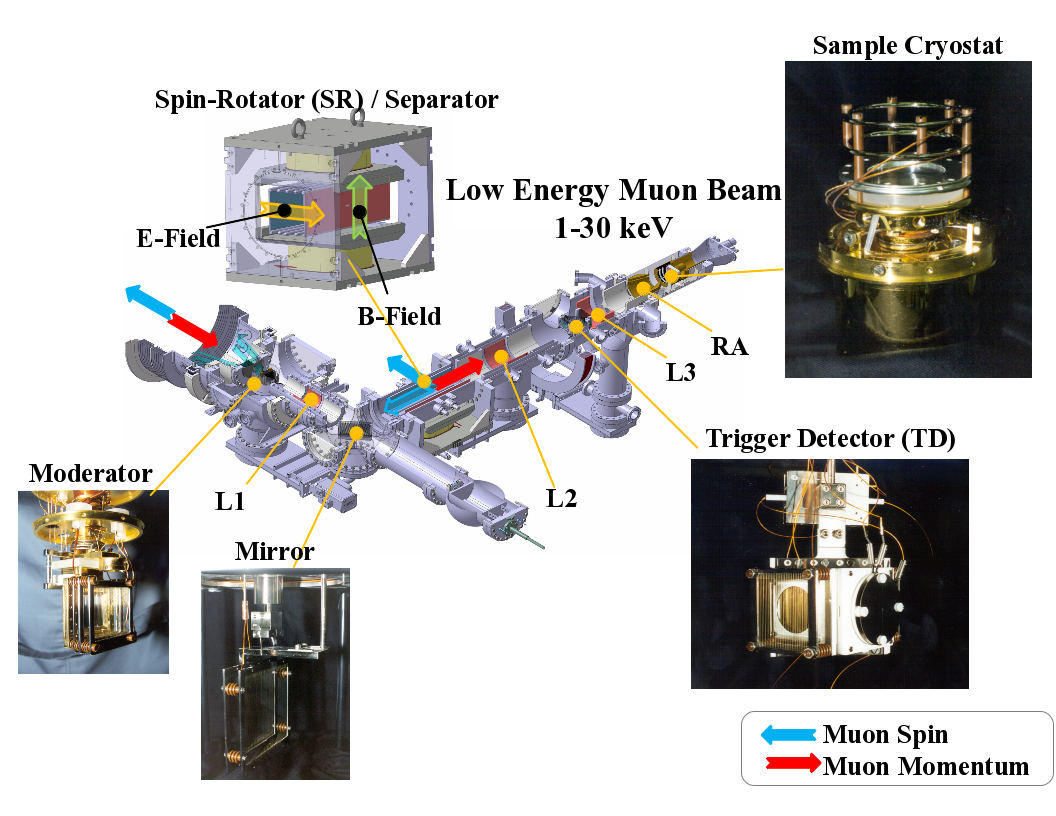
Figure 2.1: A schematic of the LEM beam line showing the different components starting from
the moderator until the sample cryostat.
For safety reasons and PSI’s legal responsibility, users are not allowed to enter the μE4 without being accompanied by their local contact. If you must go into the area in the absence of your local contact, please make sure that you inform him in person or by phone.
The μE4 area is equipped with two alarm systems. The first monitors radiation (X-ray or radioactive) in the area when it is not in “Red” or prohibited access mode. The second is an oxygen depletion monitor. If you are in the area and you hear the sound of an alarm then simply leave the area immediately and call your local contact. Please do not try diagnose or understand the source of the problem, just leave immediately.
High voltage (up to 20 kV) power supplies and high DC currents (up to 600 A) are used for the low energy muons (LEM) spectrometers. Liquid helium and nitrogen cryogens are used in moderator and sample cryostats to achieve the necessary low temperatures. The magnets on the LEM spectrometer generates high magnetic fields up to 0.35 Tesla. Radio frequency (RF) signals at low to moderate power levels (< 1 mW - 500 W) in the range of 0.1-30 MHz can be generated in the RF electronics of the LEM spectrometer. Various class IV lasers and high power LED light sources with wavelength between 365 nm and 635 nm and power up to 4.5 W are sometimes used to illuminate the sample in the LEM spectrometer.
All samples which are intended to be studied in the LEM spectrometer must be solid and stable in air in its the full temperature range. They should not pose radioactive, fire or any other toxic hazards at any time under normal handling conditions. Since the spectrometers operate at ultra high vacuum (UHV), gloves should be worn primarily to prevent contamination of the studied samples and cryostats, and to prevent chemical (or potentially radioactive) contamination of experimenter’s hands during mounting, removal and handling of samples.
Normal precautions with regard to high voltage or high current power supplies and cabling should be observed. The high voltage power supply for the detectors should be turned off before connecting or disconnecting the high voltage cable, and using only appropriately rated cables which are in optimal working conditions. The high current power supplies for the magnets should be turned off and disabled before connecting or disconnecting the magnets.
All cryogens should be stored in approved dewars and transferred into cryostats using suitable transfer lines. Craning helium dewars in and out of the μE4 area should be performed only by trained and authorized crane operators together with local PSI personnel. Appropriate safety equipment, i.e. suitable protective gloves and face mask, should be used when handling cryogens. Experimenters should remove any loose magnetic objects such as tools from the vicinity of magnets in the μE4 area.
Setting up the laser or light sources must be performed by the local contact. Users are not permitted to perform this procedure alone and they must wear certified laser safety glasses (provided by the local contact) if they are present during setup. The light power during setup and alignment must be kept as low as possible, in the mW range, to avoid accidental eye or skin damaging exposure. Gloves must be worn to prevent damaging or smudging glass lenses and light sources. Once the setup and alignment process is completed, the entire laser/light path should be contained within an interlocked black box, preventing hazardous exposure to high light intensities outside the LEM spectrometer.
The Experiment Leader (the main proposer) is the person primarily responsible for the safe operation of the experiment. She/He is responsible for ensuring that the apparatus and applied methods are safe, that appropriate procedures are established and implemented throughout the duration of the experiment and that members of the involved team are made familiar with the safety systems and procedures for the apparatus and experimental area. Responsibilities include ensuring that the apparatus and procedures satisfy any Swiss national or cantonal safety codes and regulations. The Experiment Leader should be aware of the training status of each experimenter in her/his team and for ensuring that they are all appropriately trained. Each experimenter is responsible for employing only safe practices while at PSI.
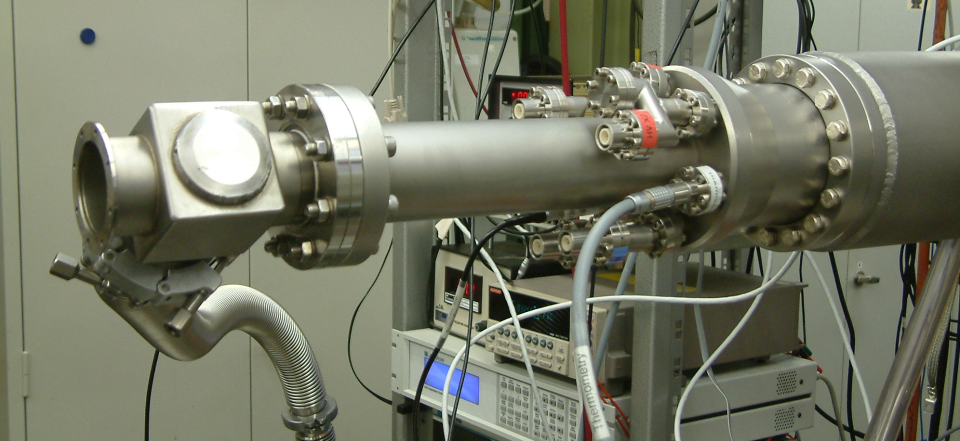
The LEM spectrometer[1, 2] is a unique instrument that enables muon spin precession and relaxation (μSR) measurements in thin films and multilayers. This is possible due to the tunable implantation energy (1-30 keV) of the muons, allowing depth resolved μSR measurements between 1-300 nm. A schematic of the LEM beam line is shown in Fig. 2.1.
Fully polarized surface muons at ~ 28 MeV/c are stopped in a solid gas moderator (see Chapter 4 for details). They are then re-accelerated using a set of grids at a high voltage (see Moderator in Fig. 2.1), focused using an Einzel lens, L1, and deflected by 90∘ using an electrostatic mirror. This deflection insures that only slow muons (at a selected energy) continue in the direction of the sample. The muons then pass through a spin rotator (SR, see Chapter 5 for details) and then into an Einzel lens (L2) which focuses the beam onto the trigger detector (TD). Due to the divergence of the beam when passing the TD we use another lens, L3 to refocus the beam into the last focusing element which we call the ring anode (RA), which in turn focuses the muons onto the a sample mounted on the cold finger cryostat or oven.
The geometry of the LEM beam line results in a muon spin polarization that is nominally parallel to the surface of the studied samples, as shown in Fig. 2.1. The muon spin can be rotated horizontally using the SR to any angle between ±90∘ relative to the surface of the sample. Two magnets can be used on the LEM spectrometer, the WEW (B perpendicular) magnet produces fields in the range -350 to +350 mT along the muon beam direction while the AEW (B parallel) magnet produces fields in the range 0 to 25 mT along the up-down direction. Therefore, one can perform zero field (ZF), transverse field (TF) as well as longitudinal field (LF) μSR measurements on the LEM spectrometer. A summary of important characteristics of the beam line, muons beam and spectrometer are summarized in Table 2.1.
| Beam line | |
| Vacuum | UHV system, ~ 10-10 mbar |
| some parts are cooled with liquid N2 | |
| μE4 beam | |
| Rate | ~ 1.9 × 10⁸ μ+/s |
| Energy | “surface” μ+ beam, ~ 4 MeV |
| Beam after moderator | |
| Rate | ~ 1.1 × 10⁴ μ+/s |
| Energy | 1 - 30 keV |
| Implantation depth | 1 - 200 nm |
| Energy spread | ΔE ~ 400 eV, Δt ~ 5 ns |
| Polarization | ~ 100% |
| Beam spot | ~ 12 mm diameter (FWHM) |
| Sample environment | |
| Temperature | 2.5 - 500 K |
| Magnetic field | 0 - 25 mT ∥ surface (AEW) or |
| 0 - 350 mT ⊥ surface (WEW) | |
| Rate | at sample ~ 4500 μ+/s |
In preparation for a LEM experiment, the following general steps are taken,
Less experienced users will be gently guided by a local contact to help them get started and run the experiment. In this chapter we give a quick and general overview on running an experiment. Further details on the operation of various aspects of the experiment are given in the following chapters.
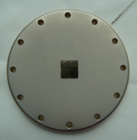
Samples for LEM measurements should be flat, plate-like such that they can be glues safely onto the flat sample plate. The samples should be “UHV clean”, i.e. should not have any greasy or organic residues on them and should always be handled while wearing appropriate gloves. The samples are generally glued using silver paint onto a silver or nickel coated sample plate (72 mm diameter). For cryostats operating below 325 K aluminum sample plates are used, while stainless steel sample plates are used for the oven. To determine the appropriate type of sample plate for your experiment, please consult with your local contact. Note that we recommend that you prepare your sample in coordination with your local contact before the “official” start date of your experiment and at least one day in advance.
After gluing, the sample plate is mounted onto a cryostat using insulating Vespel (polyimide-based plastic) screws. When using the oven, stainless steel screws are used to mount the sample plate. Typically the cryostat/oven will be sealed with a specially designed vacuum sleeve and pumped until the start of your experiment. At the official start date of the experiment (9:30 am), the cryostat/oven is inserted into the UHV beam line and pumped to a level of < 10-8 mbar before it is cooled and measurements are started.
Once the cryostat is mounted into the beam line, one can select the appropriate magnet for the experiment. For measurements requiring a field applied perpendicular to the surface of the sample (as well as ZF measurements), we use the WEW magnet (-350 to +350 mT). On the other hand, if you require fields applied parallel to the surface of the sample, then we use the AEW magnet (0 to 25 mT). Each magnet comes with its own detector set. The magnet can be installed before or after inserting the cryostat/oven (except in the case of the LowTemp cryostat). Make sure that the positron detectors are connected after installing the magnet.
The efficiency of the moderator degrades with time, typically loosing up to 30% efficiency within a week. However, this depends on the vacuum level and sample or other out-gassing elements in the beam line, which can cause a significant drop within a short time. Therefore, we deposit a new moderator layer at the beginning of each experiment, usually during the sample pumping time. Your local contact will help you with the moderator deposition, however, we give here a short description of the process. Further details can be found in Chapter 4.
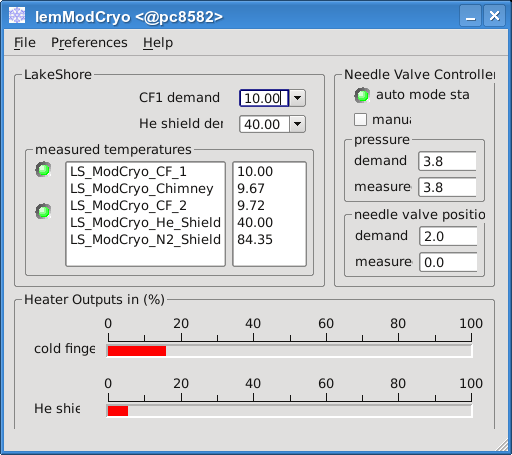
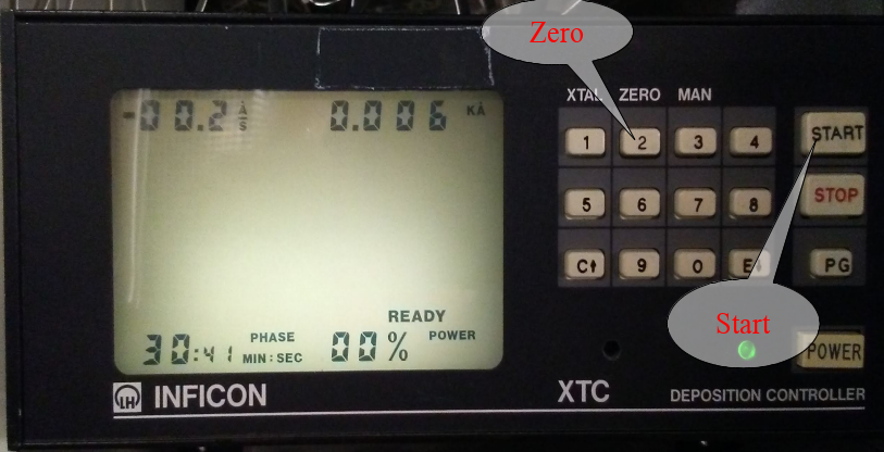
To deposit a new moderator layer, the moderator cryostat (Moddy) is warmed up to 150 K, both the cold finger and He radiation shield. The temperature is maintained at 150 K for at least 30 minutes to ensures that the old moderator layer is evaporated completely. Moddy is cooled back down to ~ 10 K on the cold finger and ~ 40 K on the radiation shield. Once the temperature is stable, a small amount of Ar gas is introduced into the moderator vacuum chamber. Some of the Ar gas freeze on the cold finger of Moddy and the thickness of the layer is monitored during this process. A typical thickness of ~ 250 nm (250 Å on the XTC monitor) solid Ar is deposited followed by a ~ 10 nm (10 Å on the XTC monitor) layer of solid N2 by introducing N2 gas into the moderator chamber.
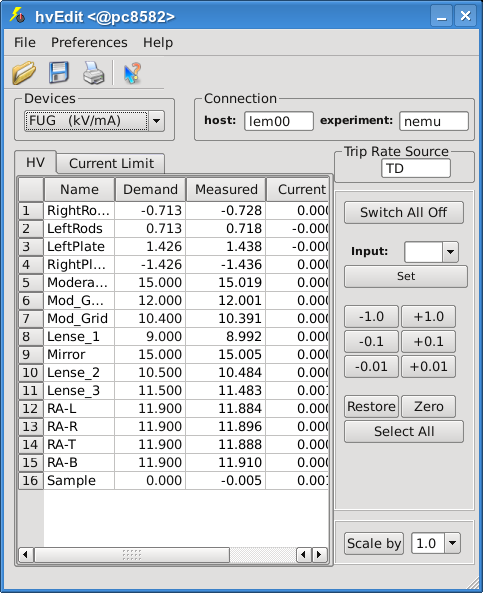
At the beginning of each year we tune the LEM beam line, optimizing the transport of muons for different kinetic energies. The results of this optimization are saved in “transport setting” files. The choice of most suitable energy for your specific experiment depends on your sample composition and thickness. Your local contact will be happy to help in deciding the right transport settings for your experiment. The task of adjusting the transport settings is then reduced to simply loading the appropriate transport setting file using hvEdit program, which you will be able to access from all desktops in the area or control cabin.
We try our best to automate all aspects of LEM, meaning that for a user, running a LEM experiment is as simple as writing a script to adjust different parameters and perform measurements. These scripts, also called autoruns, are a text file with a sequence of commands. The data acquisition systems (DAQ) performs these commands sequentially. Examples of commonly used commands are,
| TEMP | t,dt,timeout,rate |
| t | - the requested temperature in K |
| dt | - tolerance on requested temperature |
| timeout | - time out time to reach stability in seconds. |
| rate | - is the ramp rate of the temperature to reach the destination temperature in K/min. |
| FIELD | b G |
| b | - is the requested magnetic field in Gauss |
| TITLE | title |
| START | N |
| title | - the full title of the run which will be saved in the data file |
| N | - The number of positron events to be saved in the run. |
These are only a few examples to get you started, however, you can find a full list of available commands can be found in the complete LEM AutoRun Documentation. Alternatively, you may want to have a look at old autorun scripts for more examples or templates.
This chapter presents a detailed description for preparing and mounting a sample for a LE-μSR experiment. An inexperienced user will be assisted by her/his local contact throughout this process. The preparation of sample change should start well in advance of the planned change, since it involves gluing the sample on an aluminium plate which requires a few hours (preferably 6h) to dry before introducing it into the UHV beam line of the LE-μSR apparatus. Please use appropriate UHV compatible gloved during this whole process to avoid contamination of your sample or any other components that go into the UHV sample chamber. Below, we provide a detailed description of the process.
The sample can be either glued or clamped onto the sample plate. Only relatively large circular samples can be clamped. To achieve good thermal contact between the sample and the sample plate, we recommend using silver paint to glue the sample. The silver pain will be provided by your local contact. Alternatively, you may use Apiezon N grease in special cases, but this is not recommended for measurements requiring high or low temperatures. For a detailed comparison between different glues see section 9.1.
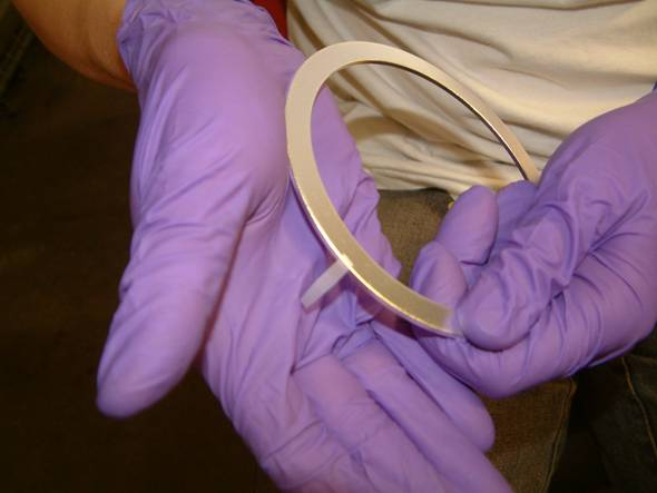
The sample plates are available in two variants, silver (Ag) or nickel (Ni) coated plates. The Ag plates are recommended if you have large samples (¿2cm diameter) or if you would prefer to work with non-relaxing background signal. The Ni plates are recommended if you have small samples and would like to suppress background signals from muons missing the samples. Consult your local contact for the best option for your specific measurement.
Once you have chosen the type of sample plate, follow theses steps to glue the sample,
Make sure that the sample is perfectly flat on the plate with no air bubbles between them.
The sample should be mounted onto a warm and dry cryostat. Typically, you will have at least one warm cryostat already available for use. However, if the cryostat is being used then it has to be warmed up before you open the UHV sample chamber. Please follow these steps below carefully (requires about two hours).
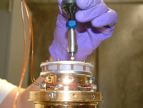
Once the cryostat is warm, you may start dismounting it by following these steps,
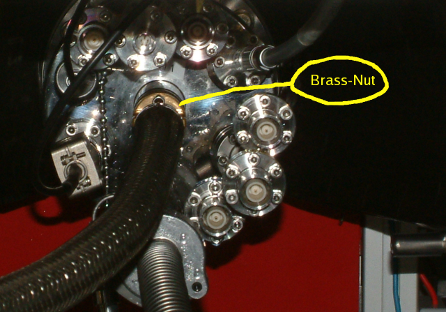
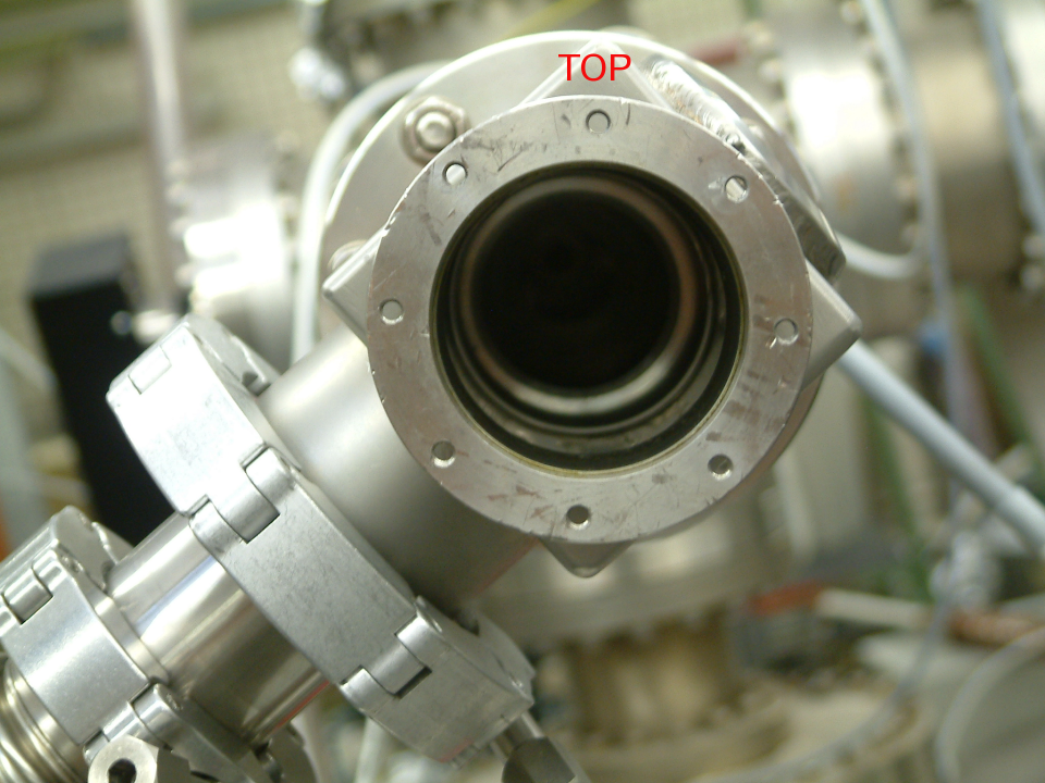
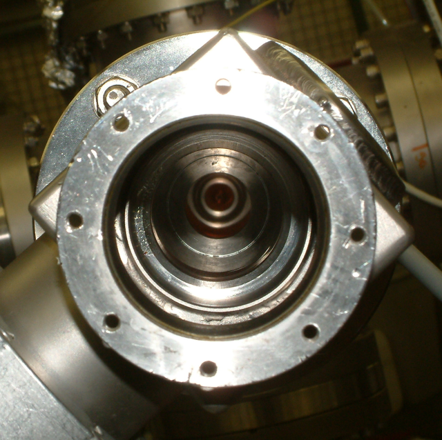
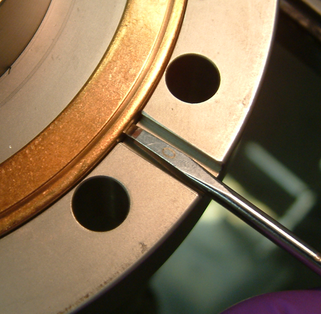
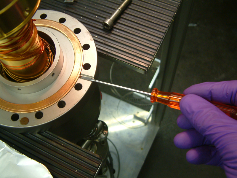
In rare cases, it may be difficult to remove the old copper gasket from the end of the beam pipe or in the cryostat flange. In this case you may need to extract it carefully using a screw driver. Insert the screw driver into the designated groove (see Figs. 3.3) and twist it gently.
Please use UHV compatible gloves when working with the sample and the cryostat. Also, avoid making any scratches on the sample plate and cryostat surfaces, since they may produce HV stability problems. Finally, always remember to connect the sample HV wire to the sample plate.
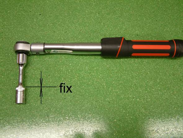
Follow carefully the steps below to mount your sample (which is already glued onto a sample plate) onto a cryostat. Whenever in doubt, do not hesitate to ask for assistance from your local contact. All tools that you will need are in/on the work bench in the clean area. Please keep these tools clean (gloves!) and keep them in the clean area.
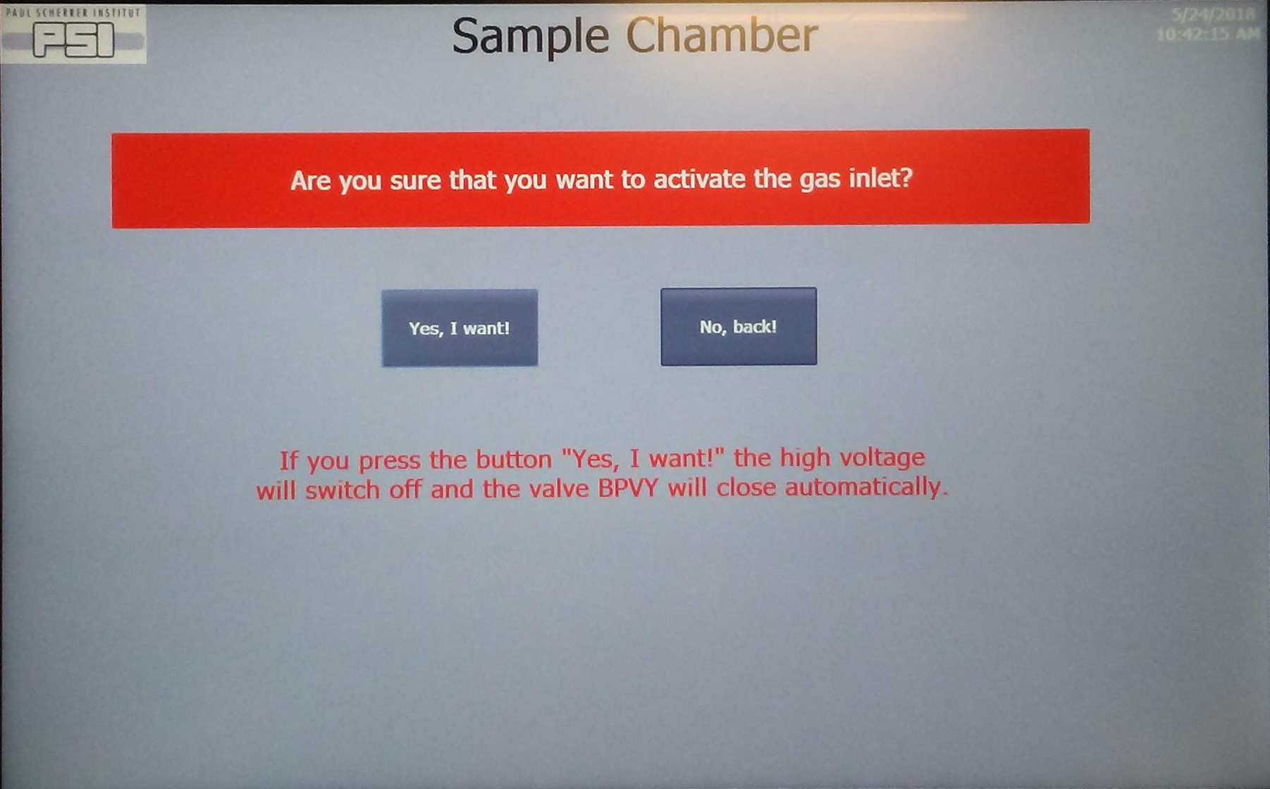
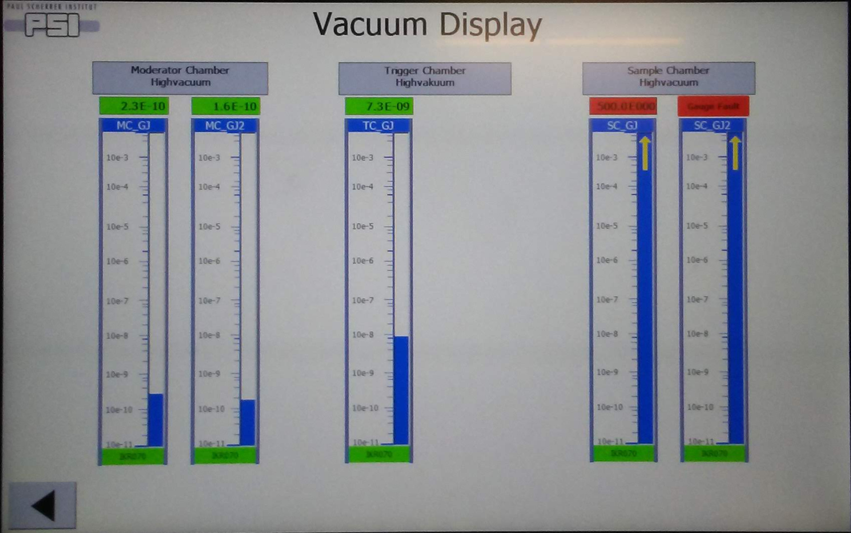
Now you are ready to remount the cryostat into the SC by following these steps,
This will get you to the “Sample Chamber” control screen, press on “No, back!” which closes the SC vent valve and takes you back to the main screen.
For a clean sample and a cryostat which was previously kept pumped in the vacuum sleeve, the pumping will take about two hours. You may open the BPVY valve (between SC and TC) only when the SC pressure, SC_GJ2, is below 8 × 10⁻⁷ mbar. This is done by clicking on the BPVY valve in the lemvac control or on the touch screen of the vacuum control. After another ~ 15 min you may start to cool down the cryostat. We recommend that you wait long enough to get to 1 × 10⁻⁷ mbar before cooling or opening BPVX. This will keep a high moderation efficiency at the moderator and prevent the formation of frozen gas layers on your samples. The latter is particularly important if you plan to work with low implantation energies/depths.
It is important to set up the correct configuration in the data acquisition (DAQ) system. This includes the name of the cryostat being used, the magnet etc. This ensures that the correct calibration tables of the thermometers are used by the temperature controller and that the correct power supply is used for the magnets. This is easily done by clicking on the “ConfigSetup” link in the navigation bar at right side of the main experiment status page, see Fig. 3.11.
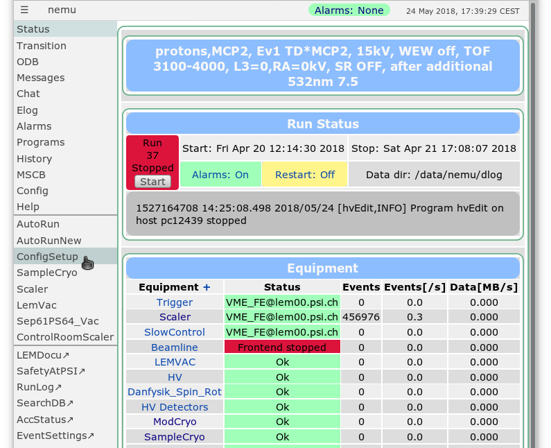
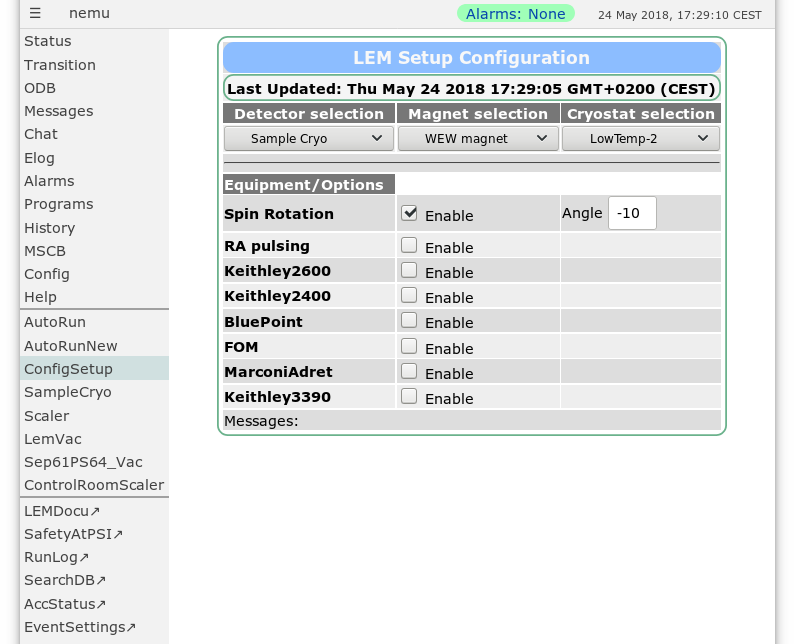
The configuration can be changed (if needed) in the following way
Having selected the new cryostat and magnet, the DAQ will automatically update all the necessary settings. You can follow and diagnose the initialization process for the new cryostat on the Midas “Messages” link in the navigation bar.
While the vacuum of the SC is being pumped, you should start preparing the cryostat for cooling and resetting the HV vacuum interlocks.
Now the system is ready to start cooling cooling the cryostat and begin with your measurements.
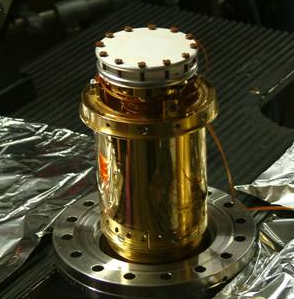
The muons in a LE-μSR experiment are moderated using a thin cryo-solid layer. The moderator is composed of a thin, structured Ag foil (~ 125 μm) on which a much thinner (< 1 μm) layer of condensed van der Waals gas is deposited[3, 4]. In order to keep the gas layer intact, it is held at a temperature below 13 K using a specially designed cryostat. The gas layer degrades slowly over time, i.e. its moderation efficiency decreases, requiring a fresh layer to be grown roughly once a week in standard experiments. The aim of this chapter is to guide you through the procedure of growing a new moderator layer. It will also provide information regarding the operation of the moderator cryostat.
A new moderator can be grown following the steps described below.
The remaining steps are optional, you may grow up to three moderators without warming up to remove a previously grown moderator. You may now go directly to Section 4.3 or follow the remaining steps to start with a fresh moderator.
Now you are ready to evaporate and grow a fresh moderator.
Different types of solid gasses can be used in the moderator, each with a different moderation efficiency and stability. The most commonly used moderator is a bilayer of N2 on top of Ar. It is also possible to use a single layer of N2 moderator. The Ar/N2 moderator is more efficient but less stable with application of high voltages compared to N2. These moderators are grown under different conditions, which are summarized in the Table 4.1.
| Moderator | Gas | Pressure | Thickness | Time | Cold | Shield |
| Finger | ||||||
| (mbar) | (kÅ) | (min) | (K) | (K) | ||
| Ar/N2 | Ar/N2 | 1E-6 | 0.230/0.012 | 3/0.5 | 10 | 40 |
| N2 | N2 | 1E-6 | 0.125 | 3 | 10 | 40 |
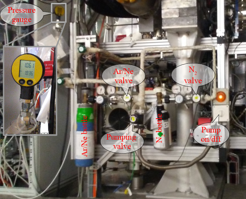
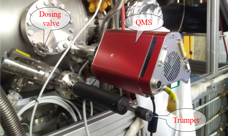
The following steps guide you through the moderator deposition process,
For example, with N2 the two highest peaks should occur at A=18,28 and 40 for H2O, N2 and Ar, respectively.
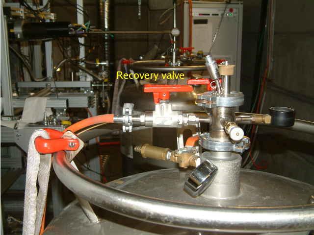
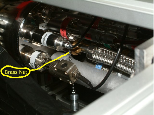
The moderator requires liquid He refilling at least once a week. This should be done before the liquid He level reaches 1.5 (check using History → Mod Cryo → LHe level). Follow these steps to refill the moderator,
In 2012 a spin rotator (SR) for the LEM spectrometer was developed to enable LF measurements. An ideal spin rotator is formed by a combination of static magnetic (B) and a perpendicular electric (E) fields which satisfy v = E∕B, where v is the velocity of the muons. This ensures that the beam is not deflected when passing through the SR. When passing through the SR, the spin of the muon is rotated by an angle θ = γBt0, where γ is the muon’s gyromagnetic ratio and t0 is the time it spends in the SR. Typically, for a surface muon beam line (~ 28 MeV/c), a rotation of 90∘ for TF measurements requires magnetic fields of ~ 0.1T and electric fields of ~ 7.5 kV/mm over a length of ~ 1.5 meters. Such requirements make the design and construction of these SRs a technically challenging task, and usually only a rotation of 40∘- 50∘ is achieved with a single spin rotator. Fortunately, the low energy of the muons after the moderator on the LEM beam line simplifies the SR requirements considerably. In this chapter we present the various aspects for the design of the LEM SR and its operation. The SR allows for a spin rotation in the range -90∘ to +90∘.
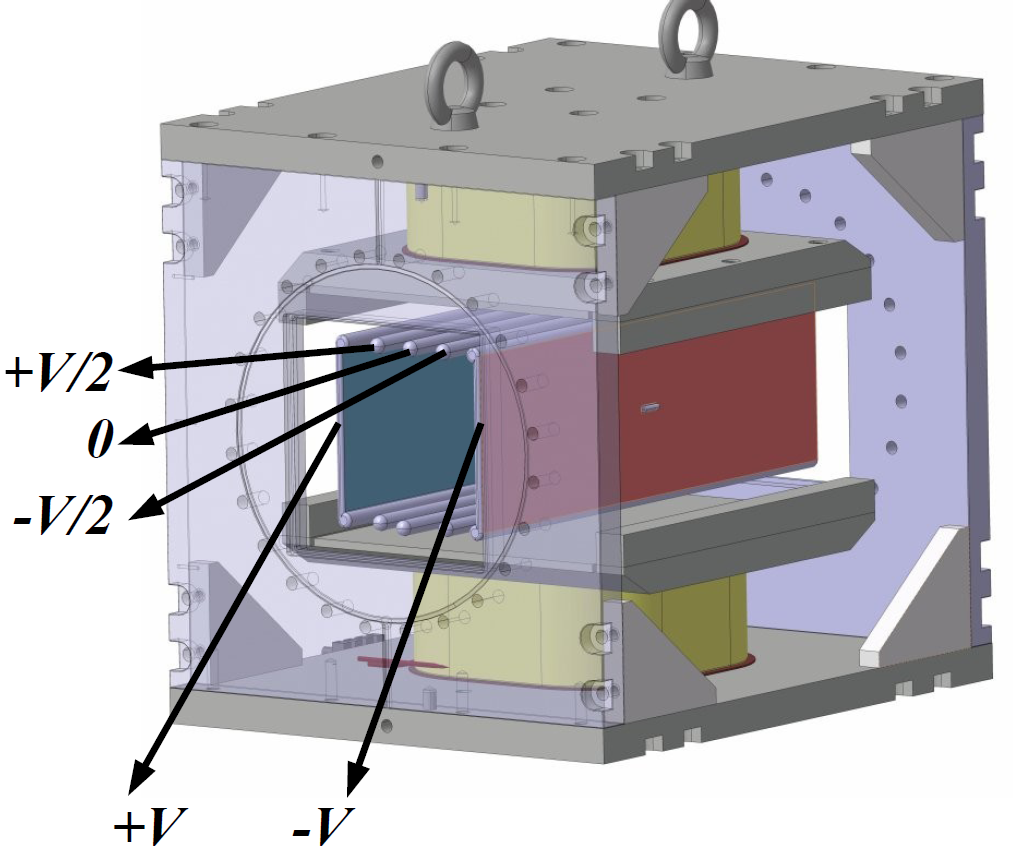
Without rotation, the initial spin of the beam as it approaches the sample, is perpendicular to its momentum due to a 90∘ bend in the beam line between the moderator and the sample position. For LF μSR measurements using the available magnets and spectrometer, one needs a spin rotator (SR) after the moderator. However, space limitations impose a small footprint of ~ 40 × 40 × 40 cm3 on the SR. Taking these limitations into consideration we designed a SR which is composed of a dipole magnet, producing a vertical magnetic field, and a set of conducting plates to produce a corresponding transverse horizontal electric field (see Fig. 5.1).
The main considerations in the magnet design were its physical length, uniformity/homogeneity and sufficient magnetic field amplitude (using a reasonable current) to achieve a full 90∘ spin rotation at typical muon energies (< 20 keV). For the electrostatic plates, we aimed at providing an electric field that compensates the deflection of the beam due to the magnetic field while maximizing beam transmission through the SR.
Figure 5.2 we plot an example of the asymmetry between the left/right detectors as a function of SR magnet current using 12 kV transport settings (potential on the moderator). The potential on the SR plates in these measurements was of course adjusted to keep the beam on axis. One can clearly see that the asymmetry follows a sinusoidal function of the current (which is proportional to the SR field and the rotation angle).
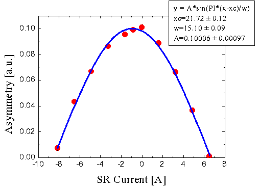
This clearly shows that continuous rotation of the muon spin in the SR between -90 and 90 degrees.
In order to simplify the use of the SR for the user, it has been calibrated extensively for
the different transport settings (8.5kV up to 20 kV). Let us denote V the absolute value
of the potential on the electric field plates, I the current in the SR magnet, and E the
kinetic energy of the muons passing through the SR. Naturally, each transport setting (E)
requires different values of magnetic (I) and electric (V ) field to achieve a certain spin
rotation. Moreover, due to the finite size of the SR and the non-ideal nature of the electric
and magnetic fields within its volume, these also depend on the required rotation angle.
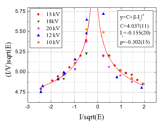
However, as can be seen in Fig. 5.3, we find that plots of I∕(V  ) as a function of I∕
 fall on the same curve for all transport settings.The logic behind this scaling is that as
the muon passes through the SR its spin is rotated by ϕ = Bt, where B is the magnetic
field and t is the time it spends in the magnetic field. This time is inverse proportional
to the velocity of the muons,
fall on the same curve for all transport settings.The logic behind this scaling is that as
the muon passes through the SR its spin is rotated by ϕ = Bt, where B is the magnetic
field and t is the time it spends in the magnetic field. This time is inverse proportional
to the velocity of the muons,  , while the magnetic field is proportional to the current
I. Therefore, ϕ is proportional to I∕
, while the magnetic field is proportional to the current
I. Therefore, ϕ is proportional to I∕ and plotting I∕(V
  ) as a function of I∕
 will give us the relation between the ratio of I∕V for a given rotation angle regardless of
beam energy, which leads to the scaling curve for all transport settings in Fig. 5.3. This
allows us to determine I and V of the SR for a certain rotation ϕ at a given transport
setting.
will give us the relation between the ratio of I∕V for a given rotation angle regardless of
beam energy, which leads to the scaling curve for all transport settings in Fig. 5.3. This
allows us to determine I and V of the SR for a certain rotation ϕ at a given transport
setting.
For the user, setting a rotation angle is a fairly simple task. Once the transport settings are loaded (i.e. the high voltage settings for the moderator and lenses), it is possible to set the muon spin angle in two different ways,
The first option is the safest and best option for spin rotation. It is also recommended that the user uses a spin rotation of -10∘ even in TF experiments. This operation mode effectively uses the SR in separation mode, i.e. filters the beam from charged ions and other contamination and reduces the number of false hits on the trigger detector.
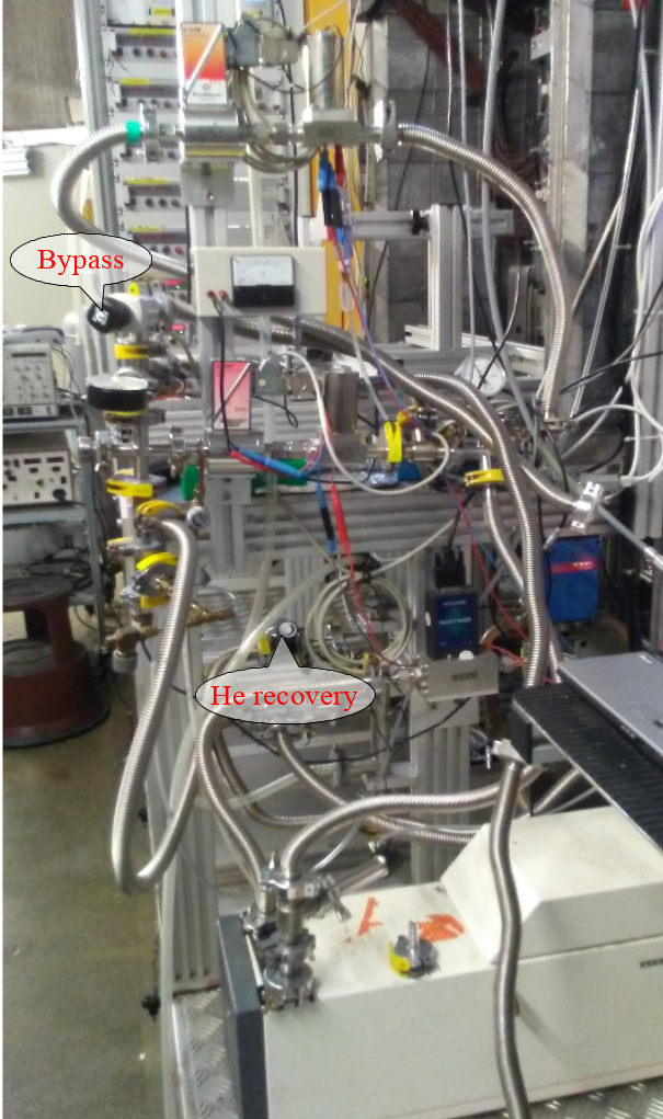
All cryostats used in the LEM sample environment are He flow cryostats, i.e. liquid He or cold He gas are pumped from a dewar through the cryostat. A heater mounted on the cold finger of the cryostat is controlled by a LakeShore340 temperature controller to provide a small amount of heating to stabilize the temperature. The amount of liquid or cold gas should be just enough to reach the desired temperature. The so-called Konti cryostats have one circuit for the cold gas reaching a base temperature of ~ 4K, while the LowTemp cryostats have two circuits. In the latter, an additional small vessel inside the cryostat acts as a phase separator, which is continuously filled with liquid He under low pressure. This feature allows the LowTemp cryostats to reach a base temperature of ~ 3K. The disadvantage of LowTemp cryostats is the complexity of their operation compared to Konti cryostats. In all cases, care has to be taken to prevent moisture from entering the cold parts of the cryostat. An immediate block (freezing) will result in hours of delay to warm up the cryostat and remove the blockage. Please wear protective gloves when working with cryogenic liquids.
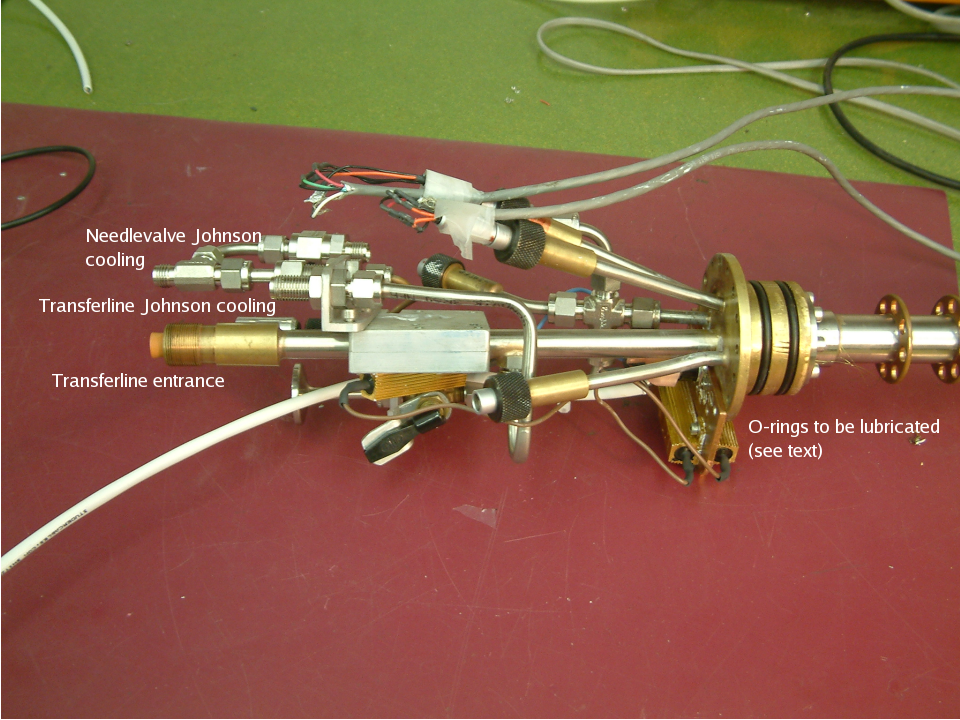
The cryostat is connected to the liquid He dewar by a transfer line, which generally has a needle valve built into it to adjust He flow through it. This valve is in the cold part of the transfer line, at the lower end of the He dewar side. To start cooling down the cryostat
The easiest way to warm the cryostat is to use the WARMUP command in an AutoRun. If you have to do it manually then
The He dewar used to cool down the sample cryostat can be changed without warming up the cryostat to room temperature. To do this,
In this section the sample environment for the LEM experiment is described. This includes the used nomenclature, a description of the different setups available and the used devices (device description, calibration tables, ranges, etc.). Before starting, we ask you to wear protective gloves whenever working with cryogenic liquids.
All cryostats used in the LEM sample environment are of the ”flow” type, that is: a dewar with liquid helium is permanently connected and a pumping system sucks the liquid helium or cold helium gas through the system. An additional heating system, connected to the LakeShore340 temperature controller supplies a small amount of heat for final temperature stabilization. The amount of liquid or cold gas should be just enough to reach the temperature, too much will -if possible- be evaporated by the heater. The so-called Konti-cryostats (for short Konti) have one circuit for the cold gas, the LowTemp type have two circuits. In the latter, there is a small vessel, called phase separator, inside the cryostat that deals with the liquid helium flow. Hence, the LowTemp’s can reach a lower temperature (~ 2 K at the base-plate), but are more difficult to operate and regulate. In all cases, care has to be taken that no moisture or air enters the cryostat while it is cold. An immediate block (freezing) will inhibit the cryostat from working and will cost you an hour or more to solve.
The Konti are the working horses for the LEM experiment. They have minimal consumption while being very robust. The typical temperature ranges (at the base-plate) of the different Konti cryostat is 3.8 K to 320 K. The upper limit is a protective measure due to indium seals in various positions in the Konti cryostats. The liquid helium consumption of a Konti is 2 l/hour (liquid) at 5 K, decreasing down to 0.06 ltr/hour at room temperature, almost following an inverse temperature curve, consumption (l/hour) = 10/T (K). Below 5 K the consumption increases more rapidly with decreasing temperature. The factory manual for the Konti’s can be found at http://lmu.web.psi.ch/docu/manuals/device_manuals/CryoVac/Konti-2.pdf
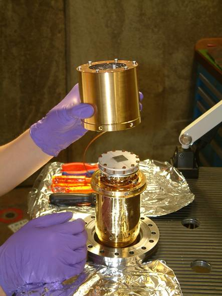
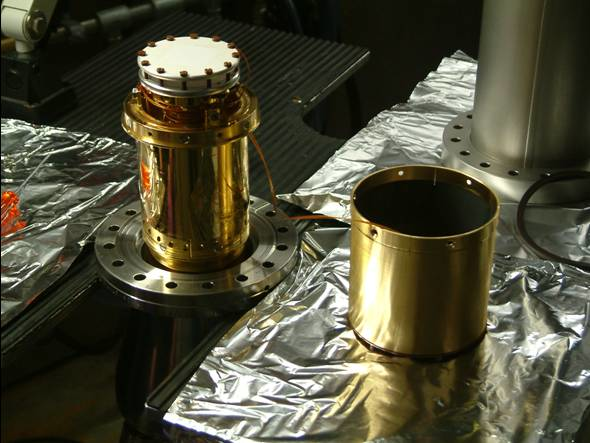
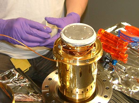
The Konti flow cryostats consist of a cold finger, surrounded by a radiation shield. The so-called base-plate is directly screwed onto the cold finger (Fig. 7.1). There is a heater of 25 Ohm wound around the cold finger and two Si-diode thermometers are mounted on the back of the base plate. These diodes are called CF1 (or D1) and CF2 (or D2), normally these are connected to A and B input channel of the LakeShore340 temperature controller. A third diode (CF3 or D3) is mounted on the radiation shield, while a fourth one (D0) is factory mounted below the cold finger. Since we need the possibility to have the sample at high electric potential (+ or - 12.5 kV), there is a 6 mm thick sapphire plate between the base plate and the sample plate. The high voltage also implies that no thermometers can be mounted on the sample plate.
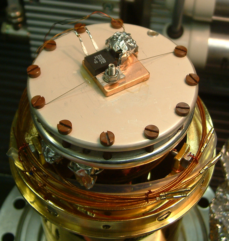
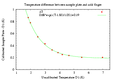
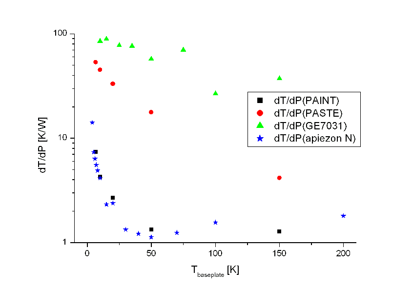
The effect of gluing the sample on the sample plate, while it is subjected to quit some heat load due to thermal radiation in the sample-chamber was measured in a separate experiment. A copper plate (25 × 25 mm2) was equipped with a heater and a calibrated thermometer as in Fig. 7.2.
The effect of different glues on the thermal contact of the sample to the sample plate can be seen in Fig. 7.3.
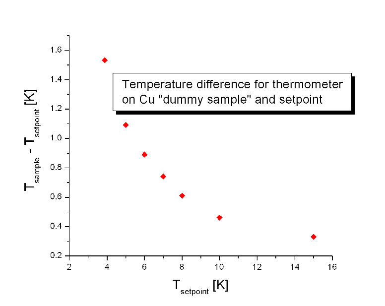
Nevertheless, be aware of the fact that the heat load on a 20 × 20 mm2 sample is of order of 0.1 W, resulting in a temperature difference between set-point as shown in Fig. 7.4. Note that for shiny samples this effect is much smaller.
The sample mounting procedure is described in Chapter 3. There is a radiation shield around the sample assembly. Inside this shield there are two guard rings, which can be put on a high electrical potential as well. However, this possibility is rarely used, but can be important when the electric field near the sample has to be decreased in order to avoid sparking. Calibration tables for the thermometers and parameters for the temperature regulation are automatically uploaded to the LakeShore340 depending on the configuration screen (Fig. 7.5).
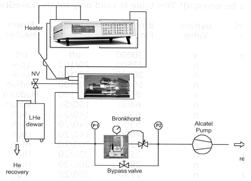
Pumping of the He gas from the Konti is done by an Alcatel Dry Pump, 20 m3/h via a Bronkhorst flow regulator. It is important to have the correct amount of flow through the cryostat to reach the demand temperature.
The He gas flow on the exhaust of the cryostat is controlled by a flow meter (Bronkhorst on the sketch) which measures the flow and regulates it via an automatic needle valve. The flow should be such that a slightly lower temperature can be reached, the heater, governed by the LakeShore340, then takes care of the last adjustments. In the Midas status page the flow is given in “Bronkhorst Units” (BH), 1 BH = 0.1 l/hour of He gas. Note that 1 l liquid helium is equivalent to 740 l gas at normal pressure and room temperature. In other words, 7400 BH is equivalent to 1 l liquid helium per hour. The flow controlled temperature regime is applicable for temperatures T > 4 K, where the relation between the flow and the temperature is given as

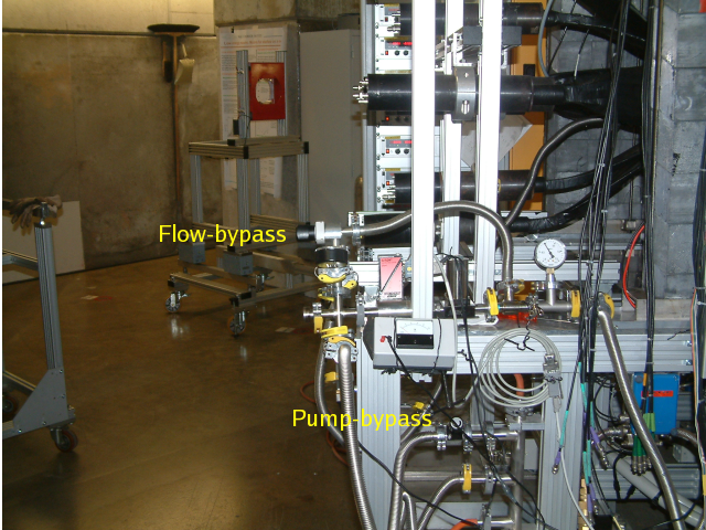
In BH-units the flow can vary between 0 and 32000. Never use a flow smaller then 600, otherwise the transfer line will warm up, which kills the flow completely. For the lowest temperature the manual bypass valve needs to be opened (Fig. 7.7).
There is a pressure gauge between the Konti exhaust and the Bronkhorst flow meter which input is fed to the LakeShore340 so that this pressure can be seen from within the Midas system. It is there for diagnostic purposes. The transfer line, bringing the liquid helium from the dewar to the Konti contains a needle valve (manually for transfer line 1 and electric for 2 and 3), which should be set such that the pressure in the pumping line is between 0.8 atm and 0.9 atm for T> 20 K, and lower (down to 0.5 atm) for lower temperatures. For the transfer line 1 (manual) this means that for an optimal operation, the needle valve should be opened about 0.3 on the scale shown on it. For the lowest temperature (T < 5 K), it can be gradually reduced to smaller values (see also FAQ).
The temperature itself is regulated by a LakeShore340 temperature controller. We are using the ZONE setting facility of the LakeShore340 in order to ease the handling of parameters like PIDs and heater range. Here is the table with the currently used ZONE settings, with the temperature given as the upper limit of a ZONE (see also the LakeShore340 manual p. 6-5, 9-42 at http://lmu.web.psi.ch/docu/manuals/device_manuals/LakeShore/). The heater range is translated to power (the Konti-1 the heater has a resistance of 25 Ohm).
| Zone | Max T | PID | Heater Range |
| 1 | 7 | 100/300/0 | 4 - 2.5 W |
| 2 | 10 | 100/200/2 | 4 - 2.5 W |
| 3 | 15 | 500/100/2 | 4 - 2.5 W |
| 4 | 20 | 500/100/2 | 4 - 2.5 W |
| 5 | 30 | 500/10/2 | 4 - 2.5 W |
| 6 | 320 | 500/10/2 | 5 - 25 W |
All the parameters of the LakeShore340 and the Bronkhorst flow meter can be set manually if needed. However, it is strongly advised to use the TEMP command of the autorun sequence (see section 2.2.5) to take over these boring jobs.
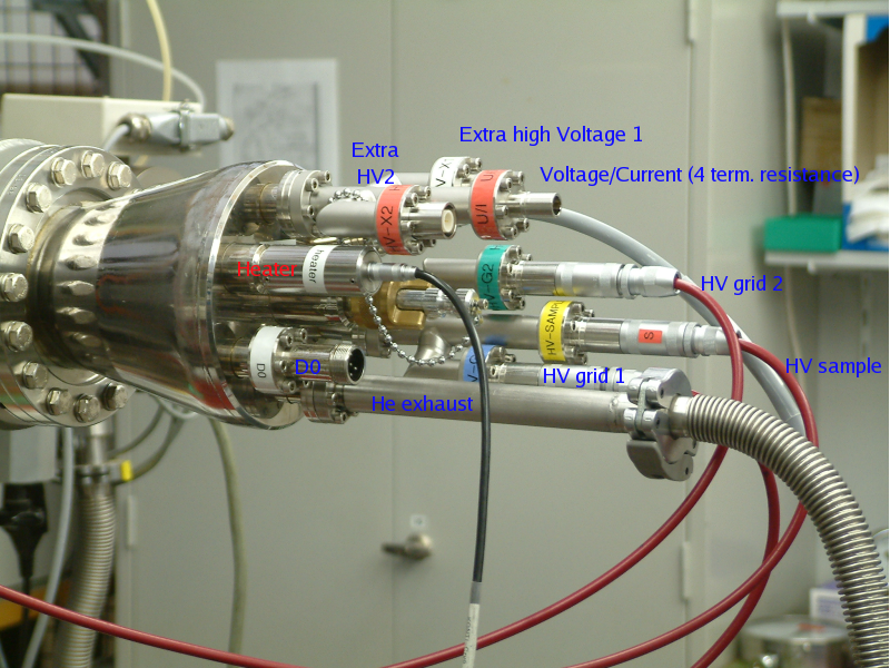
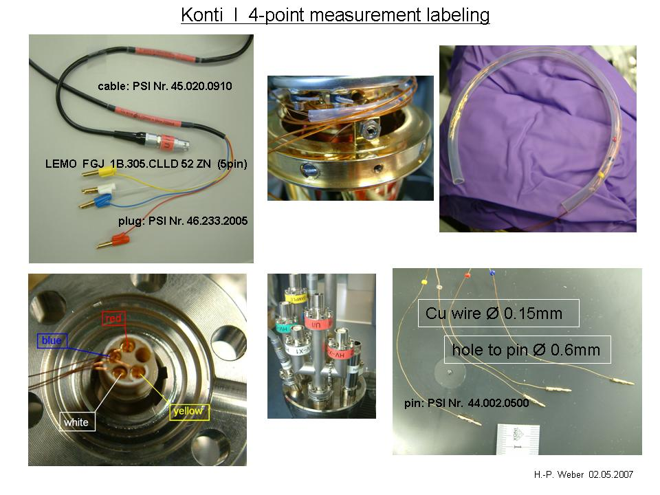
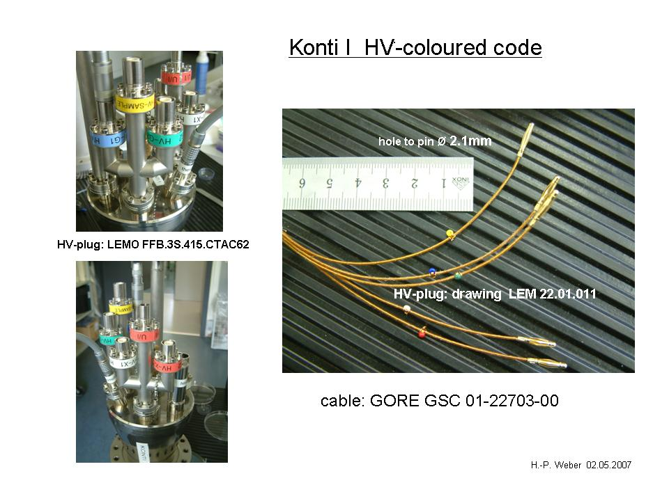
Konti-1 is the oldest of the Konti flow cryostats. Konti-1 has been equipped with extra electrical connections (at the cost of easy and quick operation) that enable the experimenter e.g. to apply electric fields to his sample and/or to measure electrical resistance at zero or at high potential, etc. The construction of the high vacuum voltage feed-troughs is such that they are in principle extendable ad infinitum.
The electrical connection are shown in Figs. 7.8-7.10.
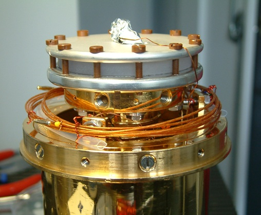
Since Konti-1 has many (high-voltage) wires running from room temperature to the cold finger, it is important to minimize the possible thermal contact these wires (in particular when they are unused) can make between the cold finger and the thermal shield. Best is to fasten the wires at the base of the thermal shield, see Fig. 7.11.
The base temperature (3.9 K on the base-plate, 4.0 K on the sample plate) has been reached with Konti-1 with flow bypass closed and a BH flow of 28000 (corresponding to 38 l/min) at a pressure of 0.6 bar. This corresponds to a helium consumption of 3.1 litre liquid He per hour. When such low temperatures have to be maintained for a prolonged period of time one better uses the LowTemp-1 or LowTemp-2, which will consume ’only’ 2 to 4 litres liquid He per hour.
The thermometers in Konti-1 are
| Zone | Max T | PID | Heater Range |
| 1 | 7 | 100/300/0 | 4 - 2.5 W |
| 2 | 10 | 100/300/2 | 4 - 2.5 W |
| 3 | 15 | 100/300/2 | 4 - 2.5 W |
| 4 | 20 | 200/200/2 | 4 - 2.5 W |
| 5 | 30 | 200/200/2 | 4 - 2.5 W |
| 6 | 90 | 400/100/2 | 4 - 25 W |
| 7 | 320 | 400/20/2 | 5 - 25 W |
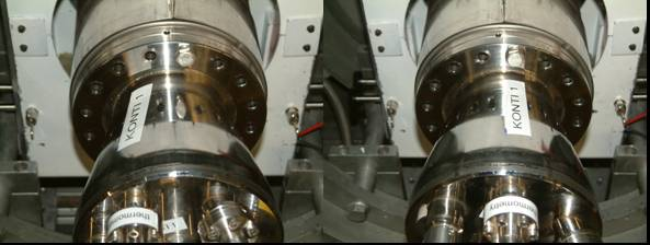
Konti-2 and Konti-3 are identical twins. They are the easy going workhorses of the sample environment and provide the basic needs for the Low Energy Muon Experiment. The temperature range is between 4 K and 300 K. High Voltage connections to the sample and the two grids are provided. Due to the low mass of the inserts temperature sweeps between room temperature and base require less than one hour.
The thermometers in Konti-2 are
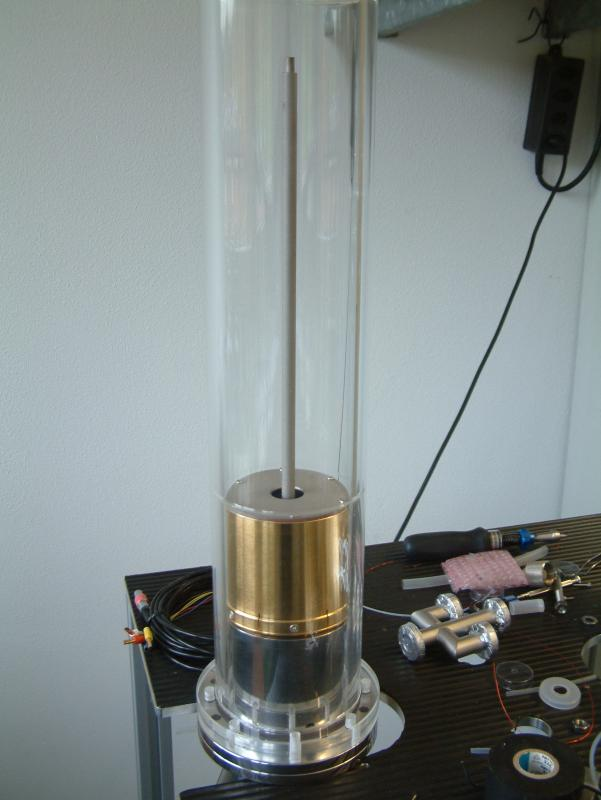
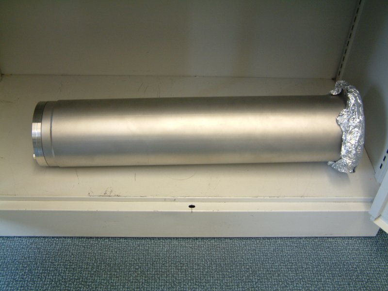
This cryostat is used mainly for small samples. The sample is mounted at the small round (10 mm diameter) copper sample plate screwed into the end of the long cold-finger tail (made of copper ~ 355 mm length 6 mm diameter). The cold finger tail is surrounded by Al tube (thermal shield) 10 mm in diameter. All the parts are covered by Ni. Konti-3 is shown in Fig. 7.12.
The cryostat is mounted using special long tube (Fig. 7.13).
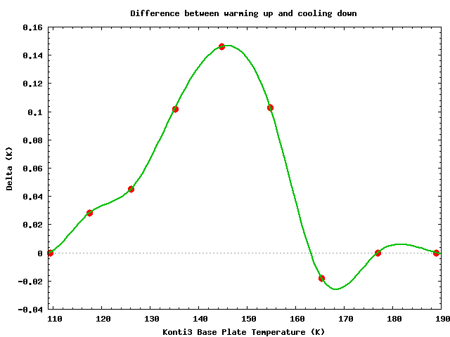
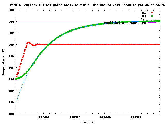
There are three peculiarities of Konti-3 related with the long tail, big thermal mass and big distance between sensors and the sample position.
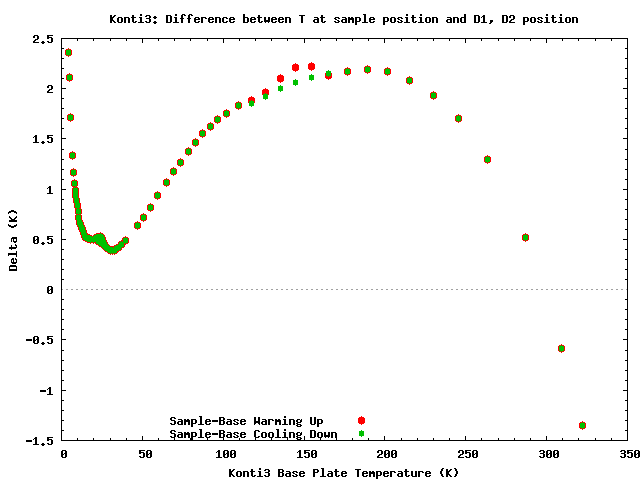
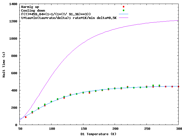
The cryostat time constant can be approximated by:
 | (7.1) |
In the autorun one has to put the WAIT command with rather big value as a parameter, e.g.
WAIT 1200
The wait time depends (in the first approximation) on the Konti-3 time constant tau, the ramping
rate, and the temperature tolerance delta. This can be estimated by:
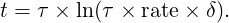 | (7.2) |
The practical (recommended) WAIT time for a ramping rate of 1 K/min and δ of 0.5 K (where δ is the maximum deviation from the set point and the real temperature) is shown in Fig. 7.16 by magenta line.
The thermometers in Konti-3 are
The Bronkhorst parameters for the Konti-3 are:
The Konti-4 setup is identical to the one of Konti-2 (see Section 7.3.2). The thermometers in Konti-4 are:
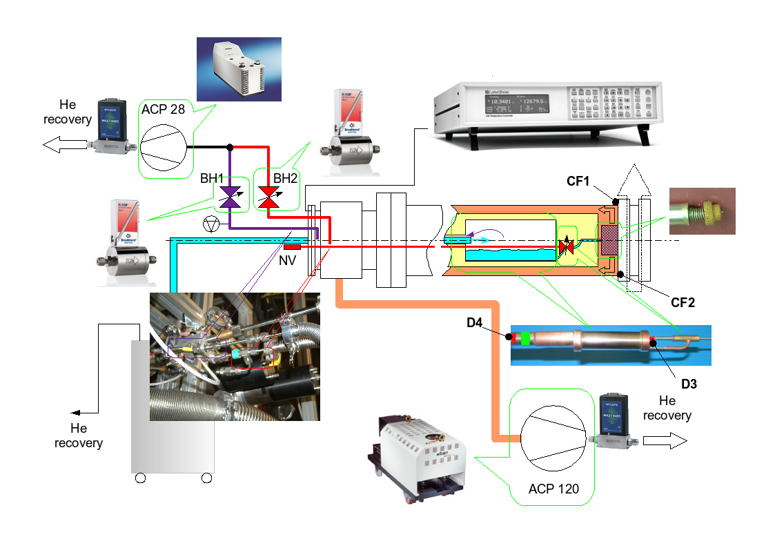
The LowTemp-2 consists of a long and hollow high-vacuum insert (Fig. 7.18) which ends in a cold finger with base-plate and sample mounting assembly. A flow cryostat can be inserted in this chamber (Figs. 7.19).
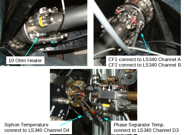
The cold gas or liquid from this flow cryostat then run along the inside of the cold finger, thereby cooling the sample. The heater again is mounted on the cold finger, this time of 10 Ohm resistance (MAXIMUM CURRENT = 1 A); the thermometers are on the back of the base-plate as in the Konti’s. When mounting the flow cryostat insert into the UHV part and the UHV part into the sample chamber, take care that the holes for the screws of the MANGO insert are pointing upward and that the big helium pumping line is pointing down, 45∘ to the left, since otherwise it will collide with the photo-multipliers.
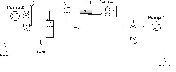
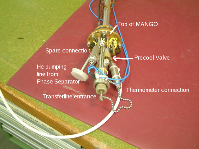
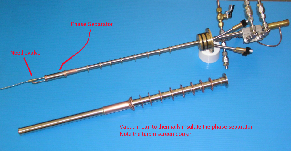
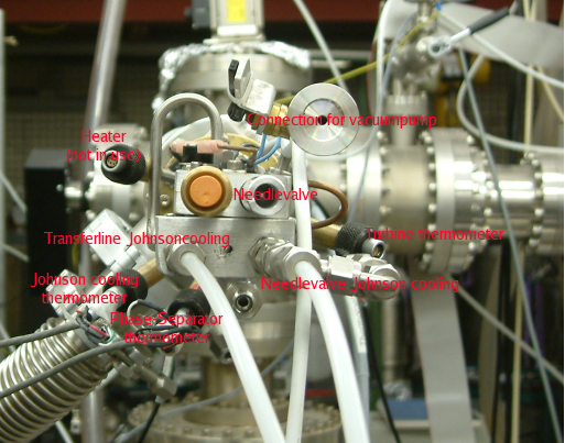
The MANGO insert has a so-called phase-separator which holds liquid helium of 4.2 K (or colder). At the bottom of the phase-separator is a capillary with a needle valve. This capillary ends in the hollow high vacuum insert just behind the inside of the cold finger. By pumping this space liquid helium is sucked at of the phase separator and evaporates at low pressure (1 Torr), and thus at low temperature (1.2 K). In order to keep the phase separator at the desired 4.2 K the incoming helium is also evaporated directly and pumped by the secondary pump. The MANGO cryostat has been designed to reach the lowest temperature possible at the lowest helium consumption, but is not able to regulate temperatures between 1 K and 6 K, since the needle valve and the phase-separator are in thermal contact with the gas pumped from the space in the insert. Heating the cold finger then results in warmer gas -> a warmer needle valve -> larger helium viscosity -> smaller flow -> less cooling power -> higher temperature -> still warmer gas -> etc. The connection diagram is shown in Fig. 7.20 and the different parts at the room temperature side on Fig. 7.21.
Note that the phase-separation depends on gravity: the top must be upwards when using the MANGO cryostat (Figs. 7.21 and 7.22).
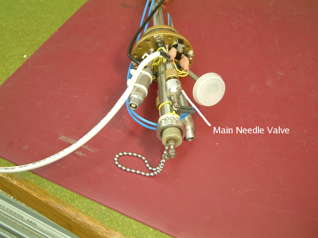
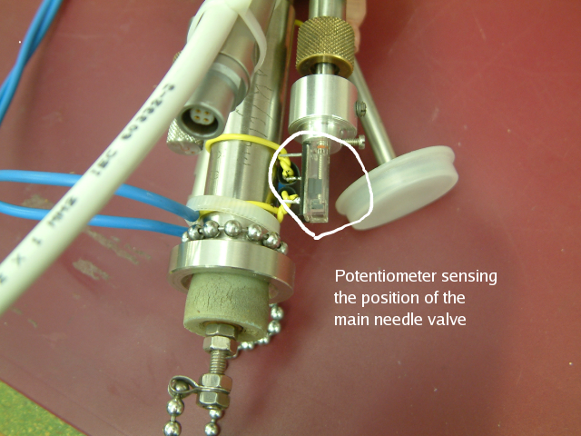
The final position of the main (=lower) needle valve is rather crucial for the correct operation of MANGO, that is low temperature at moderate helium consumption. Therefore, a multi-turn potentiometer has been mounted on the shaft of this needle valve. The potentiometer is connected to the potentiometer cable of the transfer line needle valve (Fig. 7.23). It’s position is read by the SCS900, ADC1-2 (in the area) or by the LS340, channel C3 (in the tent).
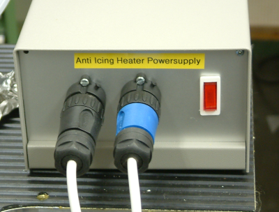
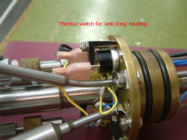
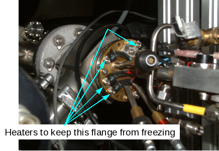
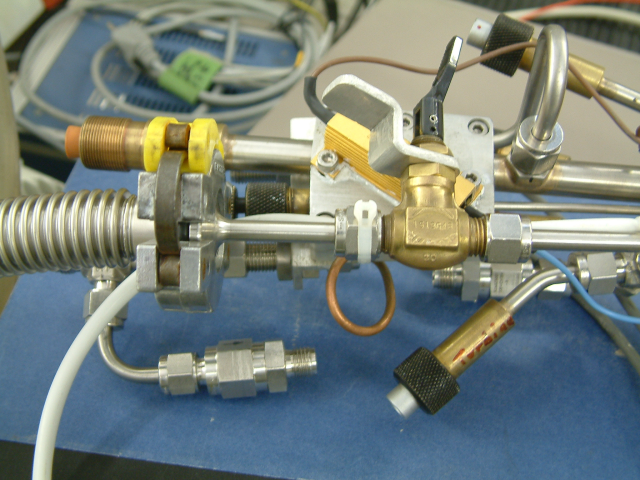
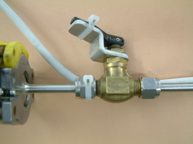
Since the MANGO cryostat is relatively short and uses about 2 l liquid helium per hour, the ’room-temperature’ part gets really cold and would collect a lot of ice. This would damage to O-rings and would inhibit the rotation of the needle valves. Four heaters (each 20 Ohm) have been mounted on the flange. They are connected, two in series and these sets parallel so that the equivalent resistance is again 20 Ohm. A thermal switch is connected in series with the heaters. The thermal switch closes below 13∘C and opens above 30∘C. The anti-icing heater should be connected to the anti-icing-heater-supply (Fig. 7.24).
The maximum voltage on the MANGO heaters is 40 Volt, the pin layout of the supply is such that this voltage is automatically connected (Fig. 7.25).
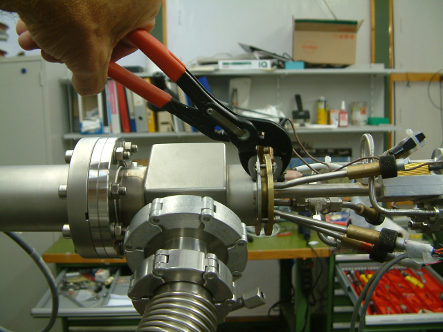
The insert has been designed and built at the University of Birmingham. It had to be designed within the restrictions of the LEM UHV beam line. Different views of the LowTemp-2 cooler are shown in Figs. 7.26 to 7.29.
Additionally, the back flow of the helium from the phase-separator is now used to pre-cool the transfer line and the needle valve. A new sinter improves the heat contact between the cold finger and the cold liquid/gas coming from the phase-separator. A turbine shaped section in the return line improves the cooling of the radiation shield of the UHV insert.
Installation of LowTemp-2 is almost the same as that of MANGO, but with a few important differences.
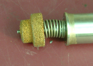
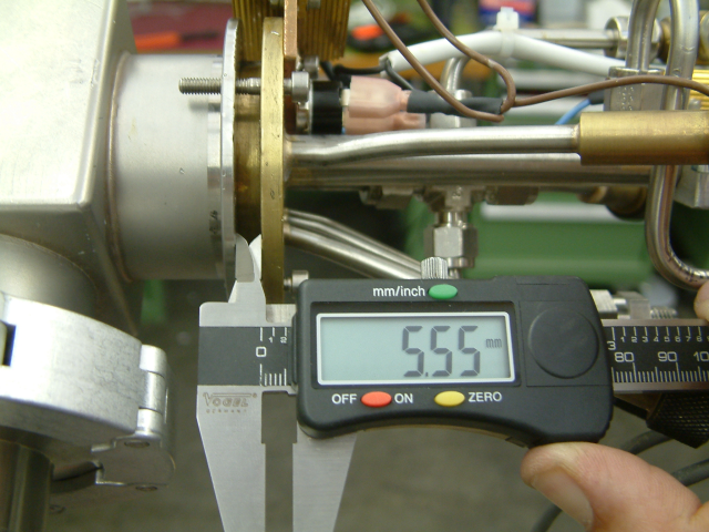
The distance should be 5.55 mm, not more and never less (Fig. 7.31).
The maximum voltage on the LowTemp-2 heaters is 60 Volt.
This cryostat operates in two modes; low and high temperature modes. The low temperature mode covers the temperature range 2.7 - 20 K, while the high temperature mode covers the temperature range 20 - 270 K. We start by describing the low temperature mode.
In this mode the temperature is stabilized by the LakeShore340 heater only. To start working in this mode, cool down the cryostat following these steps
Wait until the temperature of the phase-separator is below 4.2 K and the sample is below 4 K (after about 10 - 15 minutes from the initial cooling), then:
Some typical operation values are shown in Table 7.3.
| Time | Tsample | Phase Sep Flow | sample flow | BH1 flow | BH2 flow |
| 30 min | 2.8 | 20 l/min | 20 l/min | 12000 | 700 |
| 120 min | 2.68 | 19 l/min | 15 l/min | 10000 | 700 |
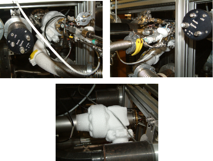
Some ice will form on the tubes, however the anti-icing heaters keep the o-rings and the needle valve knob at room temperature (Fig. 7.36).
Note that the temperature of the sample is higher then the temperature of the base-plate (Fig. 7.37).
After the base-temperature has been reached, higher temperatures, up to 20 K, can be obtained using the LakeShore340 temperature controller, without changing anything at the flow rates. The proper PID values are in Table 7.4
| Zone | Upper Zone Temp | PID | Heater Range |
| 1 | 8.5 | 250/400/1 | 4 - 0.86 W |
| 2 | 20.0 | 100/400/1 | 5 - 8.6 W |
| 3 | 60.0 | 250/400/1 | 5 - 8.6 W |
| 4 | 320.0 | 250/50/1 | 5 - 8.6 W |
Although the LowTemp-2 has been designed for the use at low temperatures, normal operation, without changing anything the in flow and NV settings, is possible up to room temperature. If one wishes to run at temperatures above 20 K, go the high temperature mode in which the cryostat is operated as a mere flow cryostat.
Note that the flow values quoted above are correct for T~ 20 K. At higher temperature these will generally be lower. This mode is mostly useful for measurements while warming up. However, in an autorun one can run in this mode going up and down in temperature between 20 - 150 K. When the temperature is higher than 150 K, cooling down to low temperature will require an increase in the Bronkhorst flow. For example, you can cool down from room temperature to 20 K by setting the Bronkhorst to a value of 9000. Once the required temperature is reached, this should be reduced back to 1800 for normal temperature stabilization.
Although it is recommended to use a 250 litre He dewar so that a dewar change during the experiment can be avoided, it is possible to use 100 litre dewars (the typical life-time is about 27 hours) and to change the dewar while LowTemp-2 is rather cold.
Bear in mind that the vacuum space has to be pumped about twice a year. This can be done by connecting the vacuum pump connector (Leybold KF6) to e.g. the rough pump of the vacuum unit in the tent. The same holds for the transfer line.
Remanent field after running degauss_danfysik: Bx = 0.01 G, By = -0.17 G, Bz = 0.12 G,
see http://lem00:8000/LEM_Experiment/4901.
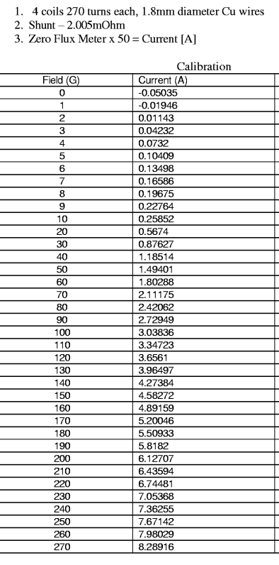
Figure 7.40 gives a field calibration table which results in

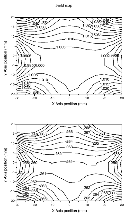
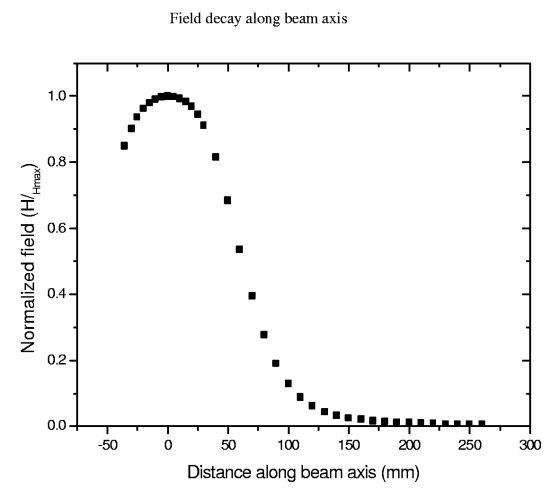
In-plane field maps at the sample position are shown in Fig. 7.41 and the field along the beam axis (Fig. 7.42).
Remanent field after running degauss_bruker: Bx = By = 0.01 G, Bz = -0.08 G,
see http://lem00:8000/LEM_Experiment/4927.
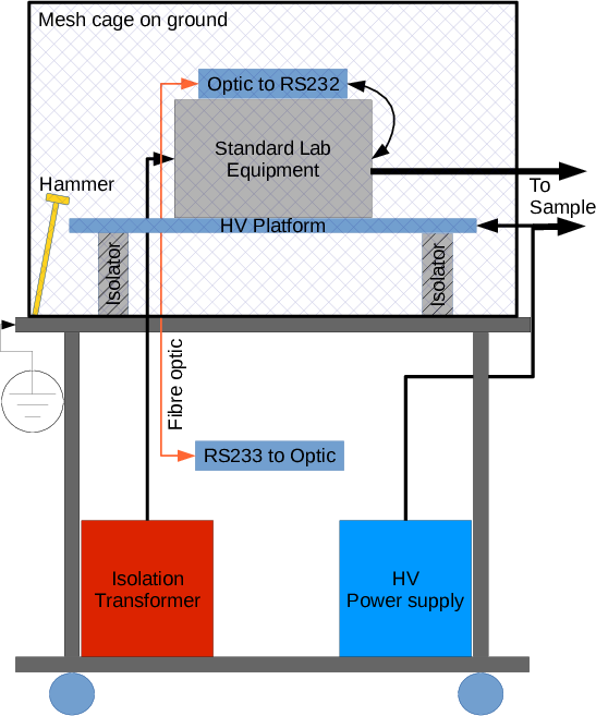
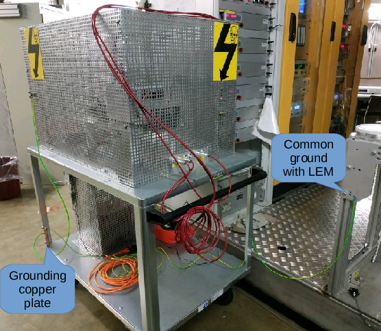
Tuning the energy of incoming muons in LEM is done primarily by applyinh a high voltage (HV) onto the sample plate. Therefore, any manipulation on the sample that requires the use of direct contacts to it becomes complicated. For example, in order to run a current through or apply an electric field on the sample, the power supply and contacts have to be on the same HV as the sample. A simple way to achieve this is to place the power supply (or any other standard lab equipment or device) on an insulated platform outside the cryostat and bias both the sample and the device by the same HV. Although the idea is simple, its application requires serious safety and reliability considerations.
A schematic of the design on the HV table is shown in Fig. 8.1. A high volatge platform is isolated from a grounded table and placed inside a grounded cage for safety. The HV platform a fed via an isolation transformer mains electricity to power the standard lab equipment, which will be connected to the sample. The sample HV bias is connected to both, the sample plate and the HV platform to ensure that they are at the exact same HV at all time. Hence, even in case of HV discharge we expect that both will remain at the same bias. We have also implemente serial RS232 communication between our DAQ and the device using fibre optic connection. This is nessesary to isolate our DAQ electronics from the HV. Other safety precations include a grounded hammer which is realease when the cage is openned exposing the HV platform. A 1 GΩ resistor is connected between the HV platform and ground to discharge the HV platform within a second once the HV is turned off. The output from the device (e.g. current or voltage leads) are delivered via suitably insulated cables to the cryostat. During operation, the electrical power which feeds the isolation transformer is interlocked with the mains electricity for the HV power supplies used for all sample chamber equipment. This ensures that the HV table and device are turned off whenever an interlock is fired due to vacuum degradation or any other issues.
Before we start, for your own safety and to comply with PSI’s safety regulations, please do this only when accompanied by your local contact.
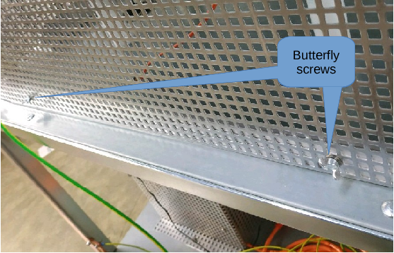
Below are a step by step instructions for connecting and preparing the HV table for an experiment. Since this setup is used only for few experiments, you will probably have to do this in preparation for your experiment.
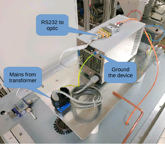
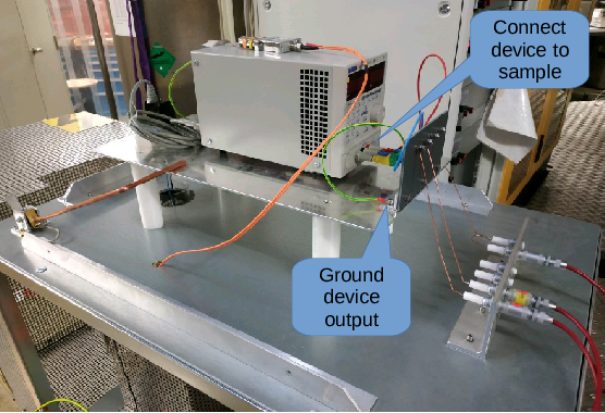
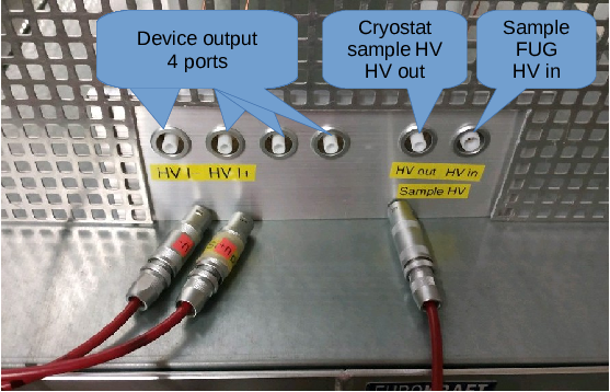
Connect the next plug from the right to the sample HV plug on the cryostat. Then connect the device ports as appropriate to the input ports on the cryostat.
At this stage, the experiment is ready to start as usual.
Figs. 9.1 and 9.2 gives an impression of the effect of different glues.
In this section the detailed update mechanism concerning the sample cryostat settings will be discussed. The ODB entry /Info/Sample Cryo defines the name of the cryostat that will be used. In sample_scfe.c frontend, there is a hotlink to this variable so that if it is changed, it will be transferred to the DD settings in the ODB, namely to /Equipment/SampleCryo/Settings/Devices/Lake340_Sample_0/DD/ODB Names/LakeShore 340 Name. The device driver ( LakeShore340.c) hotlinks the DD cryostat names and calls a routine called ls340\_cryo\_name\_changed, which is the routine which handles all the necessary changes, which are
WARNING: Please be aware of the following:
For each sample cryostat there exists a subtree in the ODB which keeps all the necessary information.
These subtree can be found under
/Equipment/SampleCryo/Settings/Devices/Lake340\_Sample\_0/DD/Cryos/CryoName where
CryoName is one of the names given in Section 3.7. The cryostat subtree is structured as
follows:
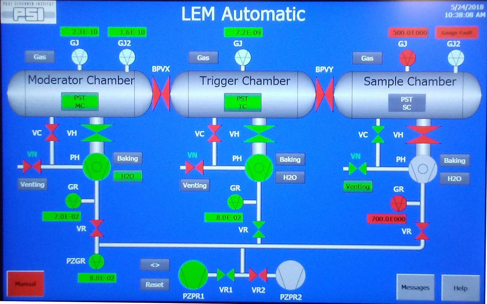
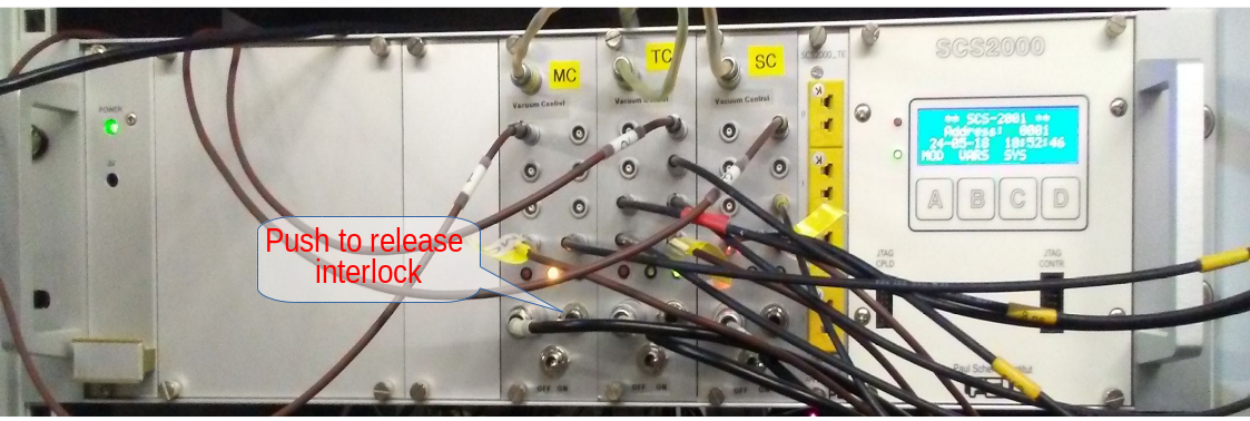
This section describes the details of the high voltage interlocks employed at the LEM beam line and spectrometer. The HV interlocks are responsible for shutting down HV elements in case of pressure increase above 1 × 10⁻⁶ mbar to protect various beam line elements. Each vacuum chamber, MC, TC and SC, has its own interlock system. For example, when the moderator cryostat is warmed up, the MC pressure may exceed the preset threshold, resulting in activation of the MC interlock with the corresponding light turning red. Once the pressure goes down below the threshold the light will turn yellow. The one can release the corresponding interlock by pressing the black push button of the corresponding interlock board (Fig. 3.13). The light will then turn green and the HVs can be reset to the correct values.
Use hvEdit to load different ”FUG_xxxxxx_2-6ug_nosample.xml” (for a 2.6μ g/cm2 carbon foil in TD) configurations with increasing transport voltage(=xxxxxx). If everything is working properly, few ions are expected to hit the Trigger Detector (TD) and the Multi Channel Plate #1 (MCP1). The dark rate of both detectors is expected to be ~ 10 counts per second. The MCP1 is a muon detector which collects muons whose energy is too high to be deflected by the mirror. Test several transport settings until your desired experimental transport settings. If at some point, the read-back values fail to meet the set-point values, stop and get help.